forked from statOmics/PSLS
-
Notifications
You must be signed in to change notification settings - Fork 0
/
Copy path03-experimentalDesign.Rmd
159 lines (107 loc) · 6.21 KB
/
03-experimentalDesign.Rmd
1
2
3
4
5
6
7
8
9
10
11
12
13
14
15
16
17
18
19
20
21
22
23
24
25
26
27
28
29
30
31
32
33
34
35
36
37
38
39
40
41
42
43
44
45
46
47
48
49
50
51
52
53
54
55
56
57
58
59
60
61
62
63
64
65
66
67
68
69
70
71
72
73
74
75
76
77
78
79
80
81
82
83
84
85
86
87
88
89
90
91
92
93
94
95
96
97
98
99
100
101
102
103
104
105
106
107
108
109
110
111
112
113
114
115
116
117
118
119
120
121
122
123
124
125
126
127
128
129
130
131
132
133
134
135
136
137
138
139
140
141
142
143
144
145
146
147
148
149
150
151
152
153
154
155
156
157
158
159
---
title: "3. Some concepts on experimental design"
author: "Lieven Clement"
date: "statOmics, Ghent University (https://statomics.github.io)"
---
<a rel="license" href="https://creativecommons.org/licenses/by-nc-sa/4.0"><img alt="Creative Commons License" style="border-width:0" src="https://i.creativecommons.org/l/by-nc-sa/4.0/88x31.png" /></a>
```{r setup, include=FALSE, cache=FALSE}
knitr::opts_chunk$set(
include = TRUE, comment = NA, echo = TRUE,
message = FALSE, warning = FALSE, cache = TRUE
)
library(tidyverse)
library(NHANES)
```
```{r pop2Samp2Pop, out.width='80%',fig.asp=.8, fig.align='center',echo=FALSE}
if ("pi" %in% ls()) rm("pi")
kopvoeter <- function(x, y, angle = 0, l = .2, cex.dot = .5, pch = 19, col = "black") {
angle <- angle / 180 * pi
points(x, y, cex = cex.dot, pch = pch, col = col)
lines(c(x, x + l * cos(-pi / 2 + angle)), c(y, y + l * sin(-pi / 2 + angle)), col = col)
lines(c(x + l / 2 * cos(-pi / 2 + angle), x + l / 2 * cos(-pi / 2 + angle) + l / 4 * cos(angle)), c(y + l / 2 * sin(-pi / 2 + angle), y + l / 2 * sin(-pi / 2 + angle) + l / 4 * sin(angle)), col = col)
lines(c(x + l / 2 * cos(-pi / 2 + angle), x + l / 2 * cos(-pi / 2 + angle) + l / 4 * cos(pi + angle)), c(y + l / 2 * sin(-pi / 2 + angle), y + l / 2 * sin(-pi / 2 + angle) + l / 4 * sin(pi + angle)), col = col)
lines(c(x + l * cos(-pi / 2 + angle), x + l * cos(-pi / 2 + angle) + l / 2 * cos(-pi / 2 + pi / 4 + angle)), c(y + l * sin(-pi / 2 + angle), y + l * sin(-pi / 2 + angle) + l / 2 * sin(-pi / 2 + pi / 4 + angle)), col = col)
lines(c(x + l * cos(-pi / 2 + angle), x + l * cos(-pi / 2 + angle) + l / 2 * cos(-pi / 2 - pi / 4 + angle)), c(y + l * sin(-pi / 2 + angle), y + l * sin(-pi / 2 + angle) + l / 2 * sin(-pi / 2 - pi / 4 + angle)), col = col)
}
par(mar = c(0, 0, 0, 0), mai = c(0, 0, 0, 0))
plot(0, 0, xlab = "", ylab = "", xlim = c(0, 10), ylim = c(0, 10), col = 0, xaxt = "none", yaxt = "none", axes = FALSE)
rect(0, 6, 10, 10, border = "red", lwd = 2)
text(.5, 8, "population", srt = 90, col = "red", cex = 2)
symbols(3, 8, circles = 1.5, col = "red", add = TRUE, fg = "red", inches = FALSE, lwd = 2)
set.seed(330)
grid <- seq(0, 1.3, .01)
for (i in 1:50)
{
angle1 <- runif(n = 1, min = 0, max = 360)
angle2 <- runif(n = 1, min = 0, max = 360)
radius <- sample(grid, prob = grid^2 * pi / sum(grid^2 * pi), size = 1)
kopvoeter(3 + radius * cos(angle1 / 180 * pi), 8 + radius * sin(angle1 / 180 * pi), angle = angle2)
}
text(7.5, 8, "Cholesterol in population", col = "red", cex = 1.2)
rect(0, 0, 10, 4, border = "blue", lwd = 2)
text(.5, 2, "sample", srt = 90, col = "blue", cex = 2)
symbols(3, 2, circles = 1.5, col = "red", add = TRUE, fg = "blue", inches = FALSE, lwd = 2)
for (i in 0:2) {
for (j in 0:4)
{
kopvoeter(2.1 + j * (3.9 - 2.1) / 4, 1.1 + i)
}
}
text(7.5, 2, "Cholesterol in sample", col = "blue", cex = 1.2)
arrows(3, 5.9, 3, 4.1, col = "black", lwd = 3)
arrows(7, 4.1, 7, 5.9, col = "black", lwd = 3)
text(1.5, 5, "EXP. DESIGN (1)", col = "black", cex = 1.2)
text(8.5, 5, "ESTIMATION &\nINFERENCE (3)", col = "black", cex = 1.2)
text(7.5, .5, "DATA EXPLORATION &\nDESCRIPTIVE STATISTICS (2)", col = "black", cex = 1.2)
```
---
# Need for a good control
- A good control group is crucial.
- To assess the effect of an intervention, we need to compare a test and control group.
- This is often not possible in a pretest/post-test design: e.g. effect before and after administering a drug without the use of a placebo group.
- Groups in an observational study are often not comparable: advanced statistical methods are required to draw causal conclusions.
- Double blinding
- We have to be aware of confounding!
- Randomized studies: random assignment of subjects in the study to the different treatment arms $\rightarrow$ comparable groups.
---
# Randomization
- Randomization completely at random (no systematic allocation).
## Simple Randomization
- Can lead to differences in the number of experimental units in each treatment arm
- in 5% of the cases we might observe an imbalance of
- of at least 60:40 in a study with 100 subjects, and
- of at least 531:469 in a study with 1000 subjects.
- This imbalance is not problematic, but causes a loss in precision.
---
## Balanced Randomization
- Equal numbers of each treatment are assigned to a block of 2 or 4 patients.
- (1) AB, (2) BA
- (1) AABB, (2) ABAB, (3) ABBA, (4) BABA, (5) BAAB, (6) BBAA
- Balanced Randomization ensures $\pm$ the same number of people in the control and the treatment arm of the experiment.
- Does not make that we have an equal number of males with and without the treatment, etc.
- In small studies, it is possible that the groups are unbalanced in other characteristics (e.g. gender, race, age ...)
- This is not problematic because it occurs at random, but, again it causes a loss in precision.
---
## Stratified randomization
- The imbalance according to for instance gender can be avoided using stratified Randomization: balanced randomization per stratum
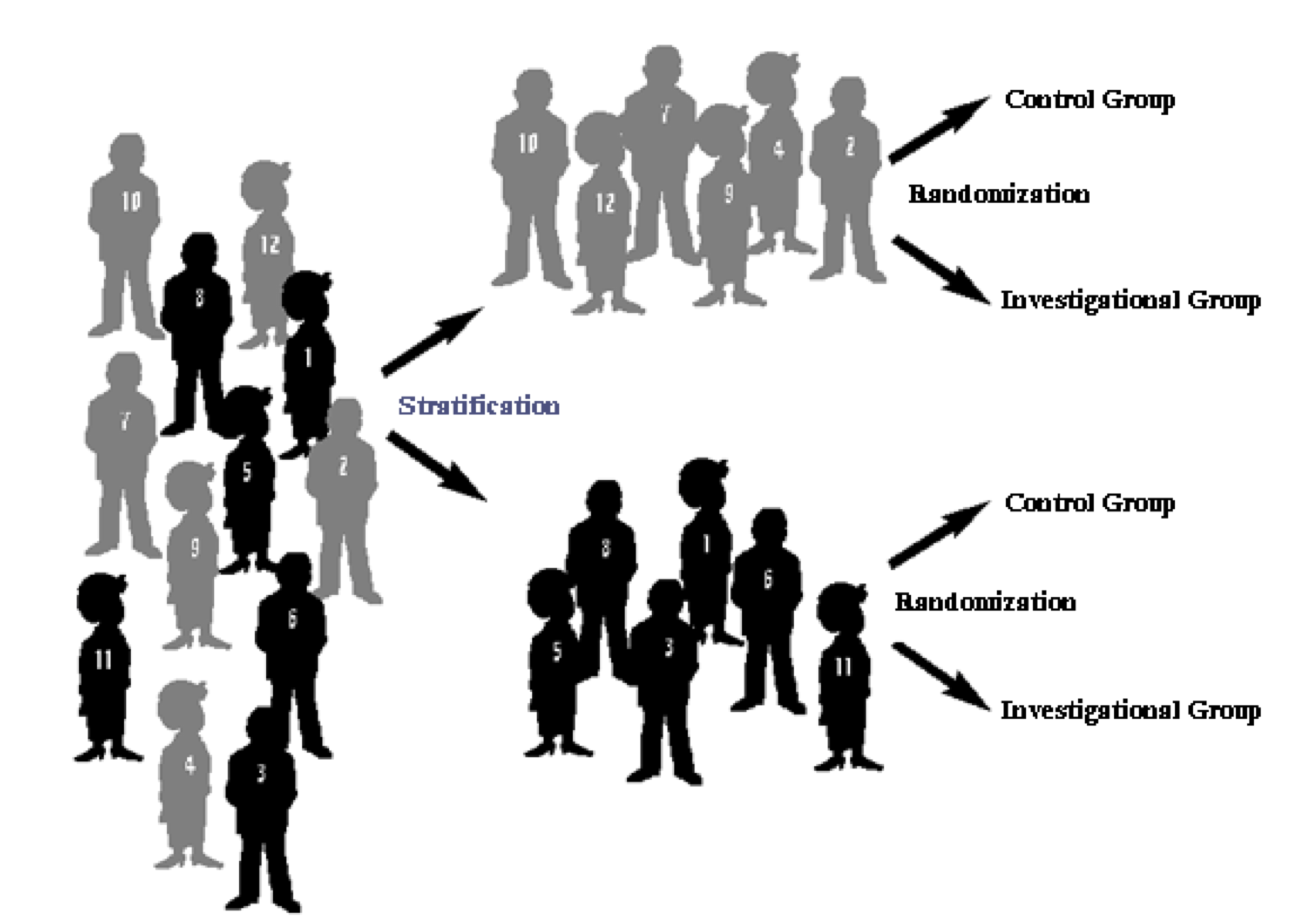{ width=50% }
---
# Sample size
- The sample size and the design are crucial.
- The larger the sample size, the more precise the results.
# Bad design example
- dm: diabetic medium, nd: non diabetic medium, co: control
- 4 bio-reps, 2 techreps/biorep
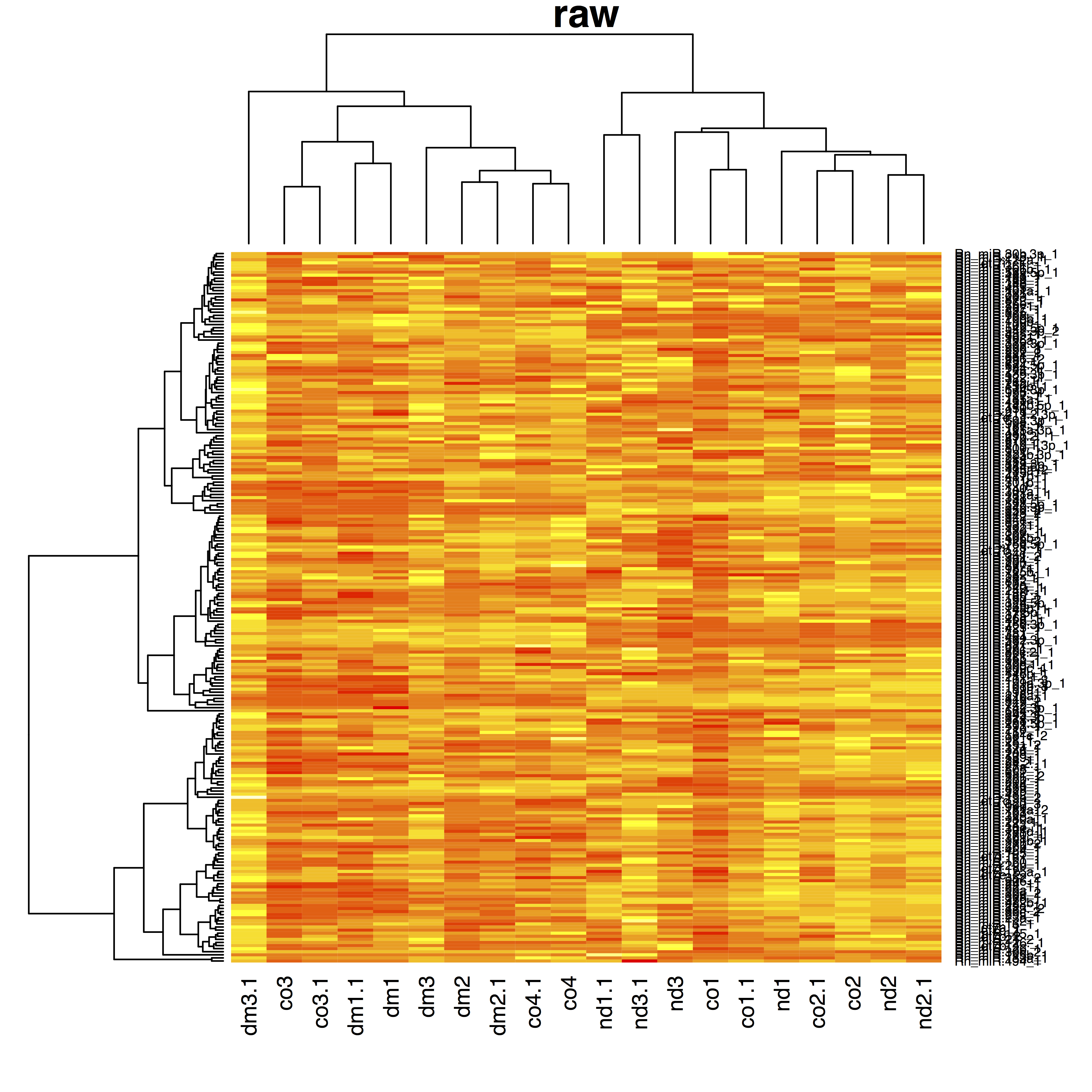{ width=100% }
- dm: diabetic medium, nd: non diabetic medium, co: control
- 4 bio-reps, 2 techreps/biorep, 2 plates A & B
- Treatment and plate almost entirely confounded
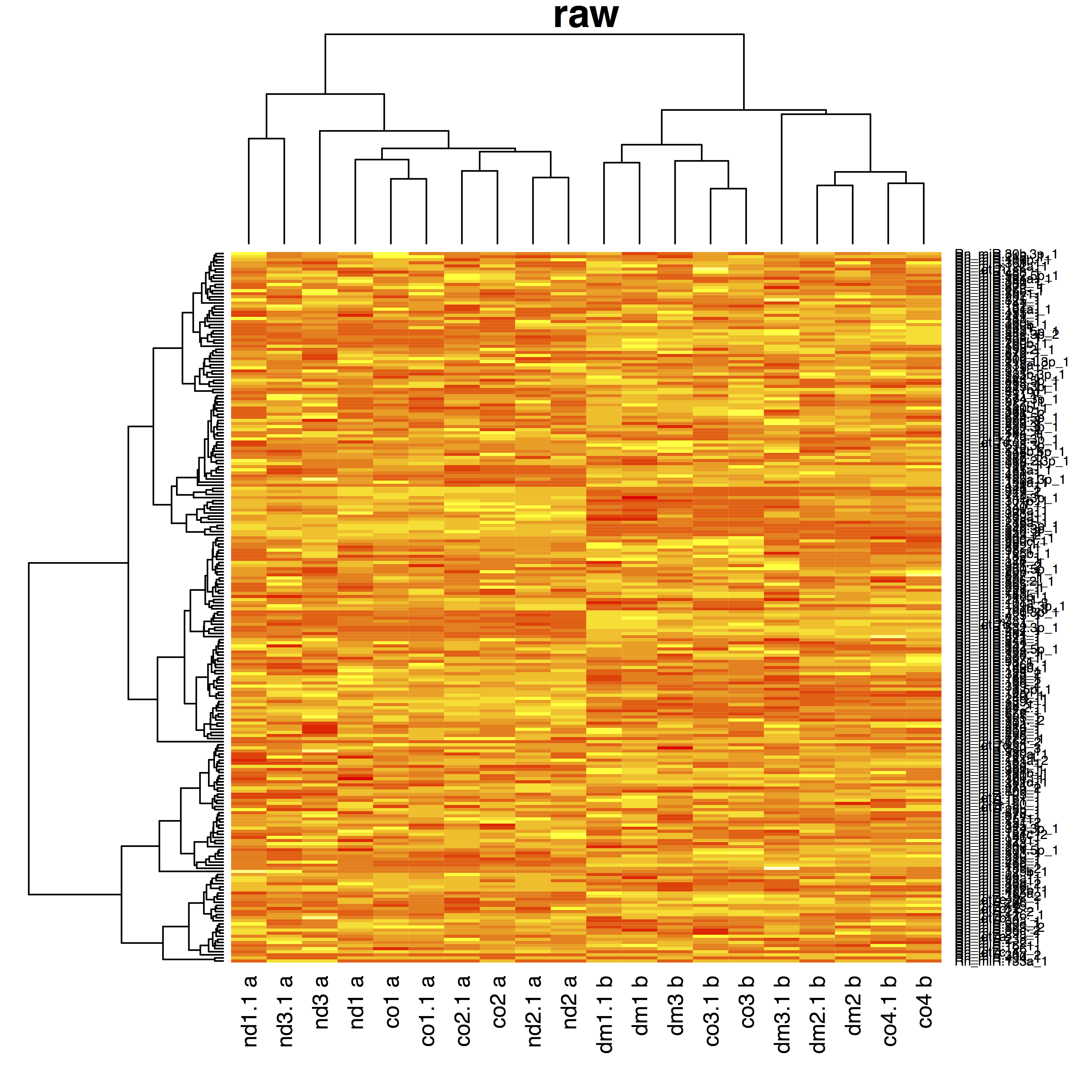{ width=100% }
---
# Wrap-up
- Sample size is very important.
- To assess the effect of a treatment, we should compare comparable and representative groups of subjects with and without the treatment (a good control!).
- In observational studies, the researcher cannot choose the treatment. It was the patient or their MD who had chosen it
- In experimental studies, the researcher assigns the treatment.
- Confounding can be avoided via randomization.
- We can also correct for confounding in the statistical analysis for the confounders that have been registered.