How do we run Kafka 100% on the object storage
This week, I’m excited to explore AutoMQ, a cloud-native, Kafka-compatible streaming system developed by former Alibaba engineers. In this article, we’ll dive into one of AutoMQ’s standout technical features: running Kafka entirely on object storage.
Modern OS systems usually borrow unused memory (RAM) portions for page cache. The frequently used disk data is populated to this cache, avoiding touching the disk directly too often, which lead to performance improvement
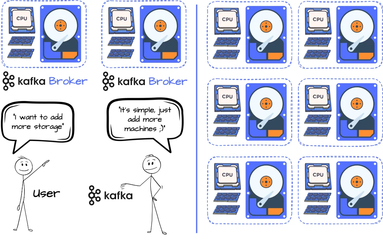
Apache Kakfa tightly-couped architecture. Image created by the author.
This design tightly couples computing and storage, meaning adding more machines is the only way to scale storage. If you need more disk space, you must add more CPU and RAM, which can lead to wasted resources.
Apache Kakfa tightly-couped architecture. Image created by the author.
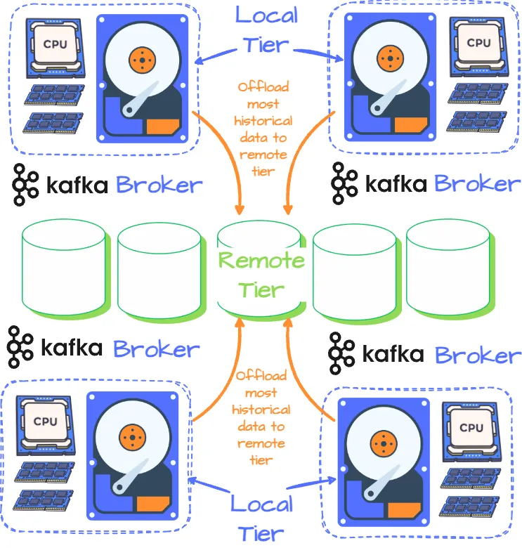
After experiencing elasticity and resource utilization issues due to Kafka’s tight compute-storage design, Uber proposed Kafka Tiered Storage (KIP-405) to avoid the tight coupling design of Kafka. The main idea is that a broker will have two-tiered storage: local and remote. The first is the broker’s local disk, which receives the latest data, while the latter uses storage like HDFS/S3/GCS to persist historical data.

The broker isn’t 100% stateless in the Kafka-tiered architecture. Image created by the author.
Although offloading historical data to remote storage can help Kafka broker computing and storage layers depend less on each other, the broker is not 100% stateless. The engineers at AutoMQ wondered, “Is there a way to store all of Kafka’s data in object storage while still maintaining high performance as if it were on a local disk?”
At the moment, AutoMQ can run on major cloud providers like AWS, GCS, and Azure, but I will use technology from AWS to describe its architecture to align with what I’ve learned from their blogs and documentation.
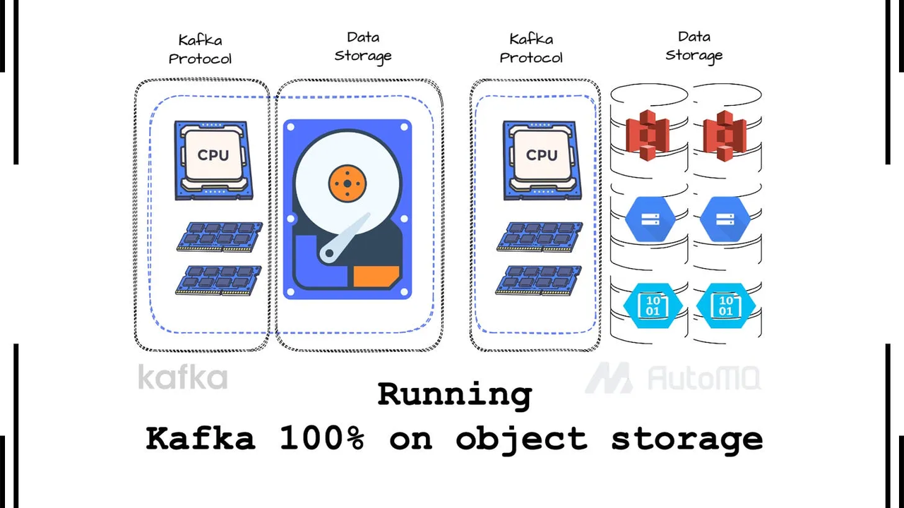
The goal of AutoMQ is simple: to enhance Kafka’s efficiency and elasticity by enabling it to write all messages to object storage without sacrificing performance.
They achieve this by reusing Apache Kafka code for the computation and protocol while introducing the shared storage architecture to replace the Kafka broker’s local disk. Unlike the tiered storage approach, which maintains local and remote storage, AutoMQ wants to make the system completely stateless.
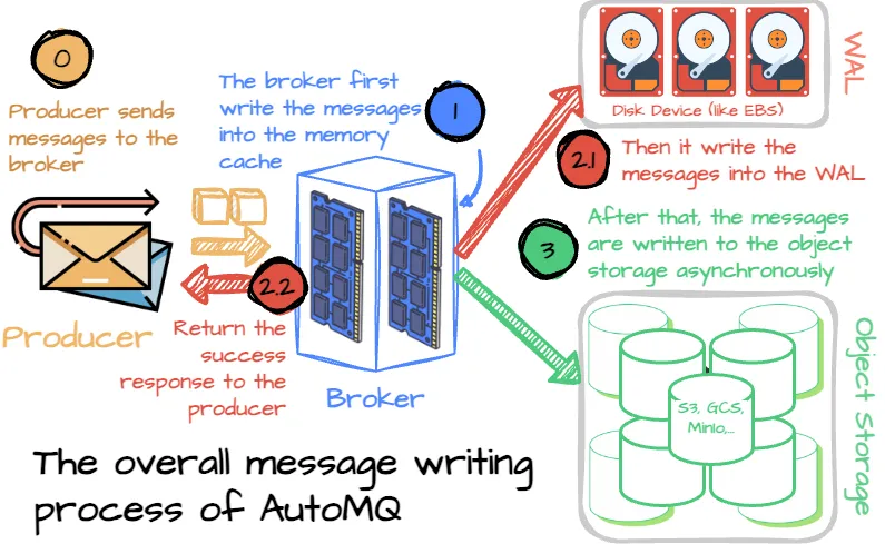
From the 10,000-foot view, the AutoMQ broker writes messages into the memory cache. Before asynchronously writing this message into the object storage, the broker has to write the data into the WAL storage first to ensure the data durability.
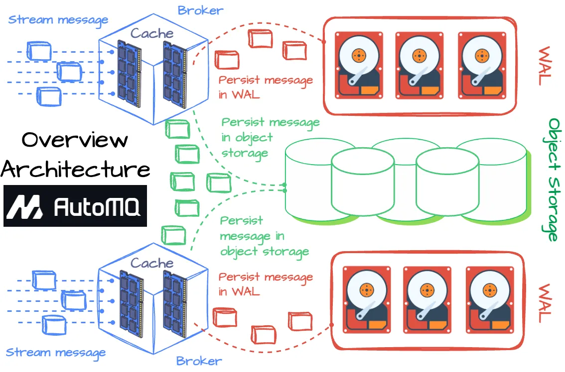
AutoMQ architecture overview. Image created by the author.
The following sub-sections go into the details of the AutoMQ storage layer.
Type of cache in AutoMQ. Image created by the author.
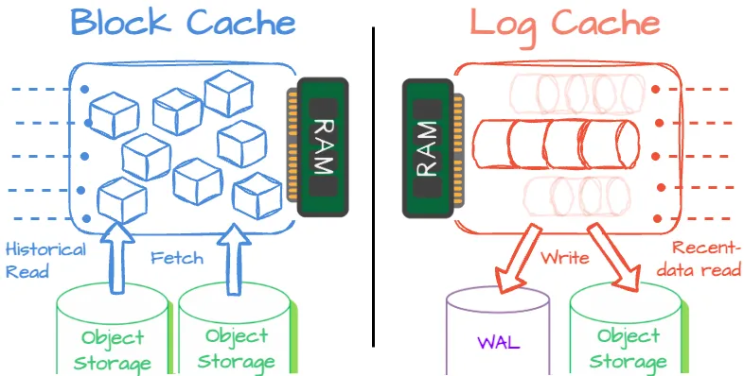
AutoMQ uses an off-heap cache memory layer to handle all message reads and writes, guaranteeing real-time performance. It manages two distinct caches for different needs: the log cache handles writes and hot reads (those requiring the most recent data), and the system uses the block cache for cold reads (those accessing historical data).
If data isn’t available in the log cache, it will be read from the block cache instead. The block cache improves the chances of hitting memory even for historical reads using techniques like prefetching and batch reading, which helps maintain performance during cold read operations.
Prefetching* is a technique that loads expected to be needed data into memory ahead of time, so it’s ready when needed, reducing wait times. Batch reading is a technique that allows multiple pieces of data to be read in a single operation. This reduces the number of read requests and speeds up data retrieval.*
Each cache has a different data eviction policy. The Log Cache has a default max size (which is configurable). If it reaches the limit, the cache will evict data with a first-in-first-out (FIRO) policy to ensure its availability for new data. With the remaining cache type, AutoMQ uses the Least Recently Used (LRU) strategy for the Block Cache to evict the block data.
The memory cache layer offers the lowest latency for read and write operations; however, it is capped by the amount of machine memory and is unreliable. If the broker machine crashes, the data in the cache will be gone. That’s why AutoMQ needs a way to make the data transfer more reliable.
Data is written from the log cache to raw EBS devices using Direct IO.
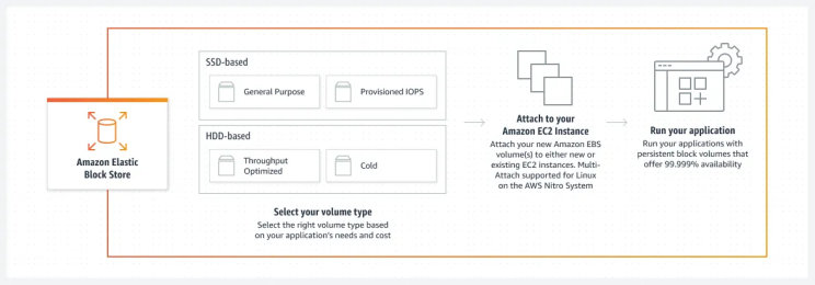
An EBS is a durable, block-level storage device that can be attached to EC2 instances. Amazon EBS offers various volume types, from SSD to HDD, allowing users to choose based on their needs. The EBS Multi-Attach feature lets you attach an EBS volume to multiple EC2 instances. We’ll revisit the Multi-Attach feature when exploring how AutoMQ recover from failure behind the scenes.
The EBS storage acts as the Write Ahead Log (WAL), an append-only disk structure for crash and transaction recovery. Databases that use B-Trees for storage management usually include this data structure for recovery; every modification must go through the WAL before being applied to the data. When the machine returns from a crash, it can read the WAL to recover to the previous state.
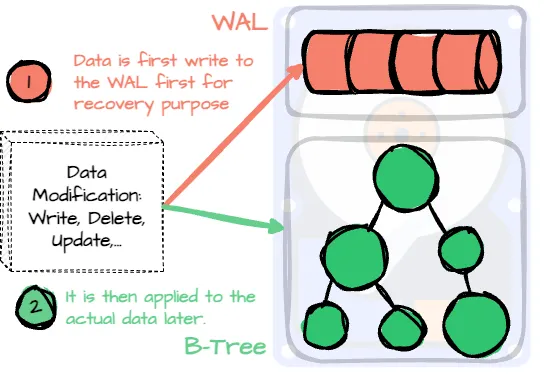
WAL in B-Tree Implementation Database. Image created by the author.
Similarly, AutoMQ treats the EBS device as the WAL for AutoMQ. The brokers must ensure the message is already in the WAL before writing to S3; when the broker receives the message, it writes to the memory cache and returns an “I got your message” response only when it persists in the EBS. AutoMQ uses the data in EBS for recovery in case of broker failure. We will get back to the recovery process in the upcoming section.

WAL in AutoMQ. Image created by the author.
It’s essential to consider the high cost of EBS, especially with IOPS-optimized SSDs type. Since the EBS device in AutoMQ serves mainly as a WAL to ensure message durability, the system only needs a small amount of EBS volume. The AutoMQ default WAL size is set to 10GB.
The object storage stores all AutoMQ data. Users can use services like AWS S3 or Google GCS for this layer. Cloud object service is famous for its extreme durability, scalability, and cost-efficiency. The broker writes the data to the object storage from the log cache asynchronously.
AutoMQ’s data files in the object storage have the following components: DataBlock, IndexBlock, and Footer, which store the actual data, index, and file metadata, respectively.
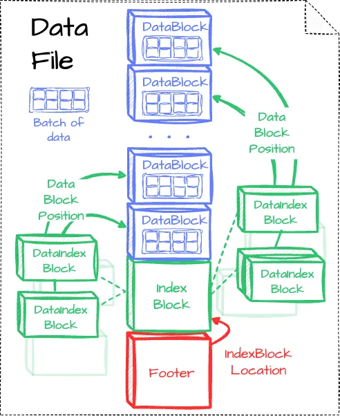
Data file in object storage. Image created by the author.
-
DataBlocks contain the actual data.
-
The IndexBlock is a fixed 36-byte block made up of DataBlockIndex items. The number of items is associated with the number of DataBlocks in the file. Information within each DataIndexBlock helps to position the DataBlock location.
-
The Footer is a fixed 48-byte block that contains the location and size of the IndexBlock, enabling quick access to index data.
The following sections will dive into the read/write operations of AutoMQ; along the way, we will understand more about how the system works under the hood.
From the user’s perspective, the writing process in AutoMQ is similar to Apache Kafka. It starts with creating a record that includes the message’s value and the destination topic. Then, the message is serialized and sent over the network in batches.
The critical difference lies in how the broker handles message persistence.
In Kafka, the broker writes the message to the page cache and then flushes it to the local disk. They don’t implement any memory cache and leave all the work to the OS system.
With AutoMQ, things got very different. Let’s take a look closer at the message-writing process:
The overall message writing process of AutoMQ. Image created by the author.
-
The producer sends the message to the broker and waits for the response.
-
The broker places the received message into the log cache, an off-heap memory cache.
Off-heap memory in Java is managed outside the Java heap. Unlike heap memory, which the JVM handles and garbage collects, off-heap memory is not automatically managed. Developers must manually allocate and deallocate off-heap memory, which can be more complex and prone to memory leaks if not handled properly, since the JVM does not clean up off-heap memory automatically.
- The message was then written to the WAL (the EBS) device using Direct I/O. Once the message is successfully written to the EBS, the broker sends a successful response back to the producer. (I will explain this process in the next section.)
Direct I/O is a method of bypassing the operating system’s file system cache by directly reading from or writing to disk, which can reduce latency and improve performance for large data transfers. Implementing Direct I/O often requires more complex application logic, as developers must manage data alignment, buffer allocation, and other low-level details
- The message in the log cache is asynchronously written to the object storage after landing in the WAL.
In the following sub-section, we will go into the details of the two processes, cache-WAL and cache-object-storage.
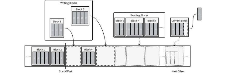
The message is written from the log cache to the WAL using the SlidingWindow abstraction, which allocates the writing position for each record and manages the writing process. The SlidingWindow has several positions:

-
Start Offset : This offset marks the beginning of the sliding window; the system already writes records before this offset.
-
Next Offset : The next unwritten position; new records start here. Data between the Start and Next Offsets has not yet been written entirely.
-
Max Offset : This is the end of the sliding window; when the Next Offset reaches this point, it will try to expand the window.
To better understand, let’s check some new data structures from AutoMQ to facilitate the write-to-EBS process:
-
block : The smallest IO unit, containing one or more records, aligned to 4 KiB when written to disk.
-
writingBlocks : A collection of blocks is currently being written; AutoMQ removes blocks once done writing them to disk.
-
pendingBlocks : Blocks waiting to be written; new blocks go here when the IO thread pool is complete, moving to writingBlocks when space is available.
-
currentBlock : The latest arrived log from the cache. Records that need to be written are placed in this block. New records are also allocated logical offsets here. When the currentBlock is full, all blocks are placed in pending blocks. At this time, the system will create a new current block.
After preparing all the prerequisite information, we will learn the process of data writing into EBS:
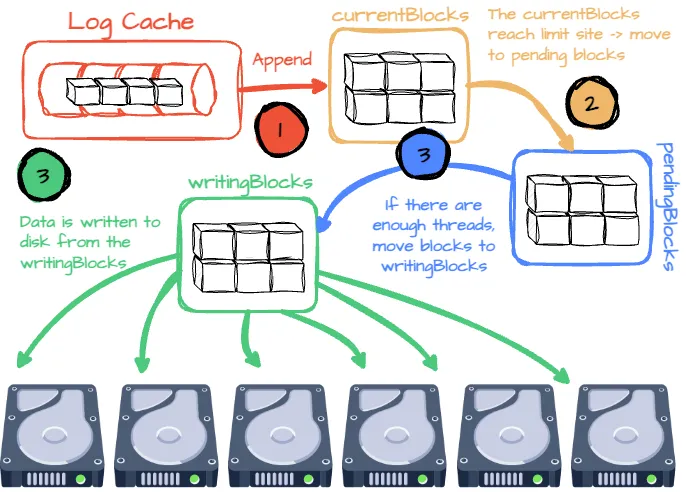
The message’s journey from the cache to the WAL. Image created by the author.
-
The process begins with an append request, passing in a record.
-
The record is added to the currentBlock, assigned an offset, and asynchronously returned to the caller.
-
If the currentBlock reaches a specific size or time limit, it moves all the blocks to the pendingBlocks. AutoMQ will create a new currentBlock.
-
If there are fewer writingBlocks than the IO thread pool size, a block from pendingBlocks is moved to writingBlocks for writing.
-
Once a block is written to disk, it’s removed from writingBlocks; the system restarts the Start Offset of the sliding window. One marks the append request as completed.
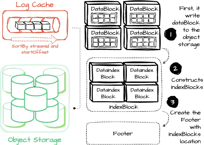
The message’s journey from the cache to the object storage. Image created by the author.
When enough data accumulates in the log cache, AutoMQ triggers an upload to object storage. The data in the LogCache is sorted by streamId and startOffset. AutoMQ then writes the data from the cache to object storage in batches, with each batch uploaded in the same order.
As mentioned earlier, data files in object storage include DataBlock, IndexBlock, and the Footer.
After AutoMQ finishes writing the DataBlock, it constructs an IndexBlock using the information from the earlier writes. Since the position of each DataBlock within the object is already known, this data is used to create a DataBlockIndex for each DataBlock. The number of DataBlockIndexes in the IndexBlock corresponds to the number of DataBlocks.
Finally, the Footer metadata block records information related to the IndexBlock’s data location.
AutoMQ Consumers start the consumption process just like with Apache Kafka. They issue an asynchronous pull request with the desired offset position.
After receiving the request, the broker searches for the message and returns it to the consumers. The consumers prepare the following request with the next offset position, calculated by the current offset position and its length.
next_offset = current_offset + current_message_length
Things got different with the physical data reading path.
AutoMQ tries to serve as much data reading as possible from memory. Initially, Kafka read the data from the page cache. If the message is not there, the operating system will go to the disk and populate the required data to the page cache to serve the request.
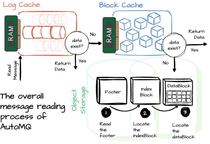
The overall message reading process of AutoMQ. Image created by the author.
Reading operations in AutoMQ follow the following paths: If the request requires recently written data, it reads from the log cache. It’s important to note that only messages already written to the WAL are available to fulfill the request. If the data isn’t in the log cache, the operation checks the block cache.
The block cache is filled by loading data from object storage. If the data is still not found there, AutoMQ attempts to prefetch it. Prefetching allows the system to load data that it anticipates will be needed soon. Since the consumer reads messages sequentially from a specific position, prefetching data can boost the cache hit ratio, improving read performance.
To speed up data lookup in object storage, the broker uses the file’s Footer to find the position of the IndexBlock. The data in the IndexBlock is sorted by (streamId, startOffset), allowing for quick identification of the correct DataBlock through binary search.
Once the DataBlock is located, the broker can efficiently find the required data by traversing all the record batches in the DataBlock.
The number of record batches in a DataBlock can affect the retrieval time for a specific offset. To address this, all data from the same stream is divided into 1MB segments during upload, ensuring that the number of record batches in each DataBlock doesn’t slow down retrieval speed.
As mentioned earlier, the role of the EBS storage is the AutoMQ’s Write Ahead Log, which helps the process of writing messages from memory to object storage more reliable. Let’s imagine a situation when an AutoMQ cluster has two brokers, A and B, each with two associated EBS storage; let’s see how AutoMQ achieves reliable message transfer:
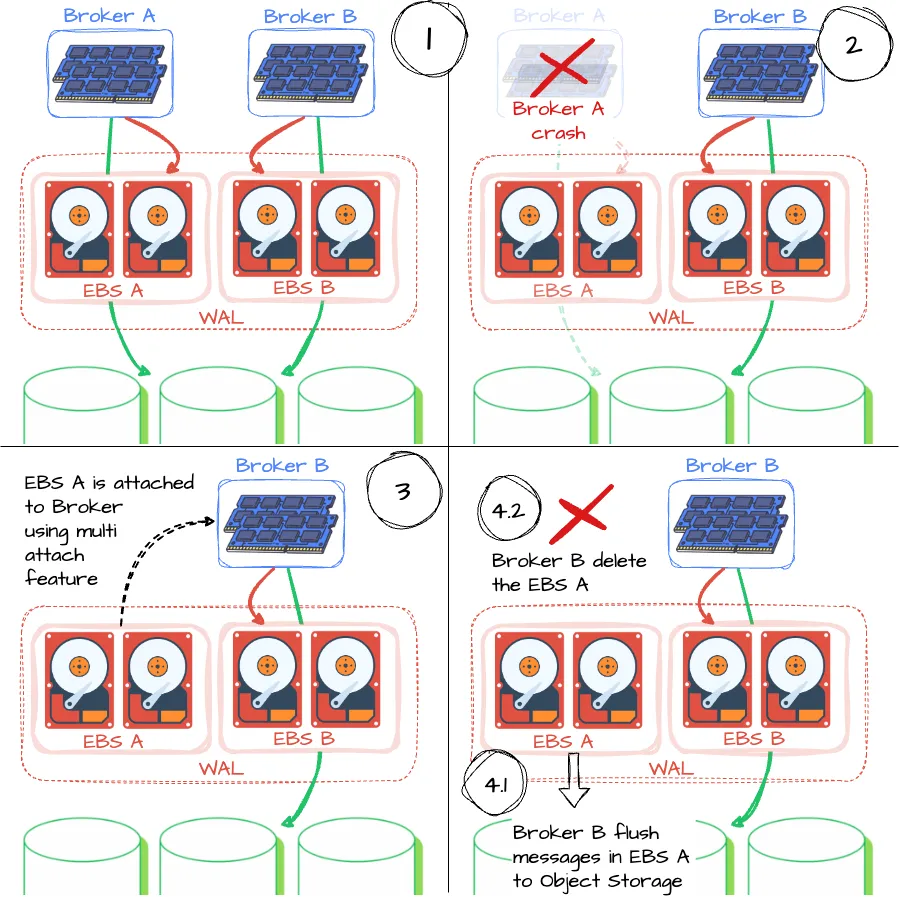
How does AutoMQ achieve reliable message transfer? Image created by the author.
-
As mentioned, a message is considered successfully received once the broker confirms it has landed in the WAL (EBS).
-
So, what if one of the brokers, says broker A, crashed? What happened with that broker’s EBS storage device? How about the EBS data that had not been written to object storage?
-
AutoMQ leverages the AWS EBS multi-attach feature to deal with this situation. After broker A is down, EBS device A will be attached to broker B. When broker B has two EBS volumes, it will know which one is attached from the idle state by tags. Broker B will flush the data of EBS storage A to S3 and then delete the volume. Moreover, when attaching the orphan EBS volume to Broker B, AutoMQ leverages the NVME reservation to prevent unexpected data writing to this volume. These strategies significantly speed up the failover process.
-
The newly created broker will have new EBS storage.
We’ll wrap up this article by exploring how AutoMQ manages cluster metadata. It reuses Kafka’s KRaft mechanism. I didn’t dive deeply into KRaft when writing the Kafka series, so this is a great opportunity to learn more about this metadata management model. 😊
AutoMQ leverages the latest metadata management architecture based on Kafka’s Kraft mode.
Traditional Kafka relies on a separate ZooKeeper servers for cluster metadata management, but KRaft eliminates ZooKeeper, simplifying Kafka and enhancing resilience. In KRaft mode, Kafka uses an internal Raft-based controller quorum — a group of brokers responsible for maintaining and ensuring metadata consistency. The Raft consensus algorithm is used to elect a leader and replicate metadata changes across the quorum. Each broker in KRaft mode keeps a local copy of the metadata, while the Controller Quorum leader manages updates and replicates them to all brokers, reducing operational complexity and potential failure points.
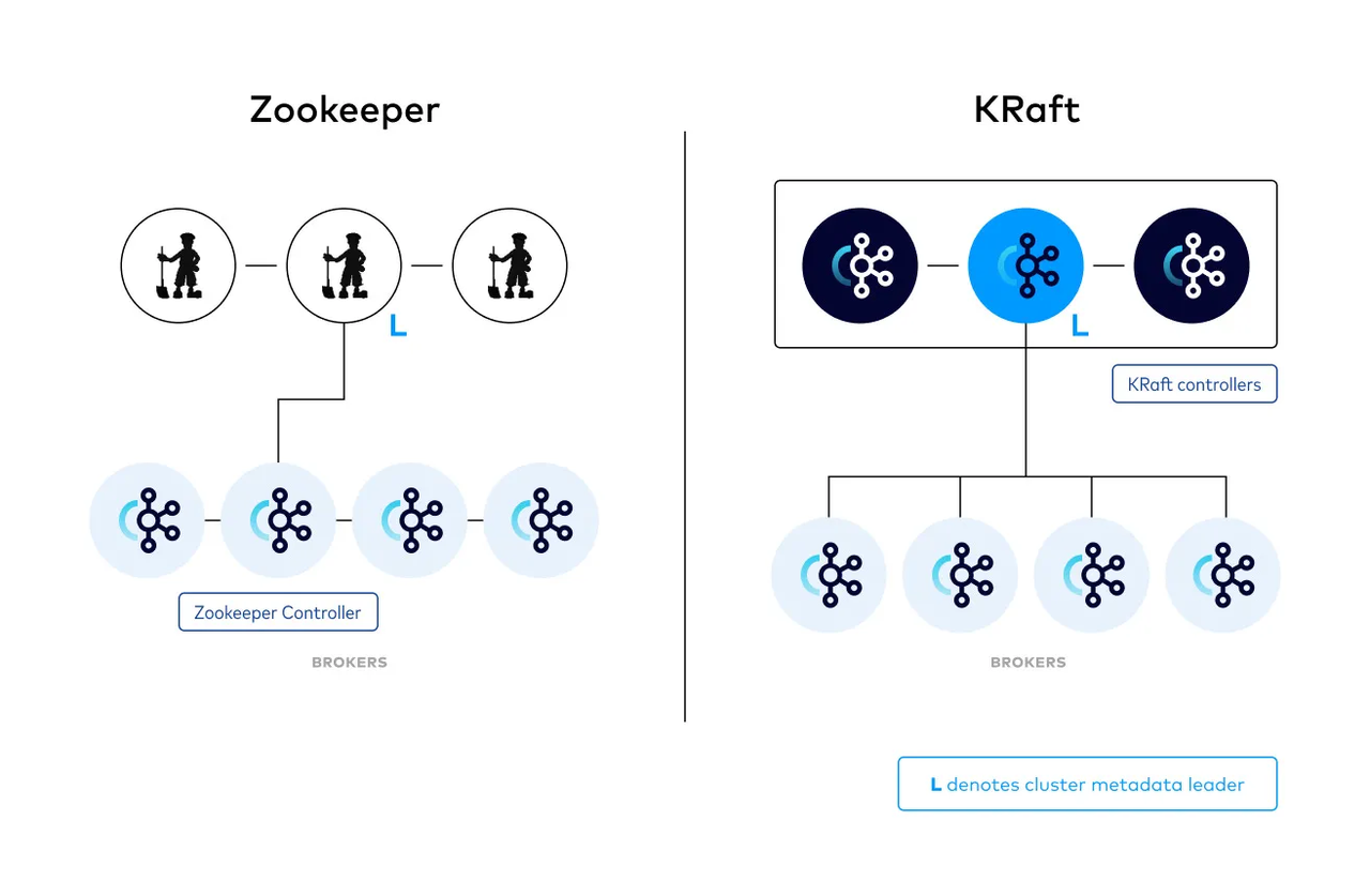
*Zookeeper Mode vs Kraft Mode. *Source
AutoMQ also has a controller quorum that determines the controller leader. The cluster metadata, which includes mapping between topic/partition and data, mapping between partitions and brokers, etc., is stored in the leader. Only the leader can modify this metadata; if a broker wants to change it, it must communicate with the leader. The metadata is replicated to every broker; any change in the metadata is propagated to every broker by the controller.
In this article, we’ve explored how AutoMQ creatively leverages cloud services to meet a critical goal: storing all Kafka messages in virtually limitless object storage while maintaining Kafka’s original performance and compatibility.
Thank you for reading this far. See you in the following article.
[1] AutoMQ Blog, How to implement high-performance WAL based on raw devices? (2024)
[2] AutoMQ Blog, Challenges of Custom Cache Implementation in Netty-Based Streaming Systems: Memory Fragmentation and OOM Issues (2024)
[3] AutoMQ Blog, Parsing the file storage format in AutoMQ object storage (2024)
*[4] *AutoMQ Github Repo